Case Study: Working with Real Data
Goal of this page
The end-to-end recipe for a real instance — the London Ambulance Service — from raw geodata and travel times through feasibility repair to a recorded chain, with links to the focused reference for each step.
The synthetic demo grid is fine for tutorials, but real workflows start from shapefiles, GeoPackages, or GeoJSON of geographic units and use real travel times. This page is a workflow guide that ties together the pieces you need, with links to the focused references for each.
The running example throughout is the London Ambulance Service (LAS) application from the FalCom paper: 4,994 LSOAs (Lower Layer Super Output Areas) of the LAS catchment (Greater London’s 5,042 minus the 48 Brentwood LSOAs LAS does not serve), annual attended-incident counts as demand, the 66 active ambulance stations as level-1 candidates, and the 21 Group HQs — each itself an active station — as level-2 candidates. The full LAS pipeline lives in the London-Ambulance-Service-System repo; this page distills the recipe.
0. The instance
Before any chain mechanics, it helps to see what the dataset actually looks like. This is the LAS case-study instance from the FalCom paper, drawn at build time with FalcomPlot’s geographic helpers. The docs ship the catchment polygons (simplified for size), the dissolved catchment boundary, and the dual-graph edge list — the latter two computed from the full-resolution geometry.
First the geographic units. plot_units draws the LSOA polygons and
the city boundary:
import geopandas as gpd
import falcomplot as fp

lsoa = gpd.read_file("_static/las_lsoas.geojson")
boundary = gpd.read_file("_static/las_boundary.geojson")

fp.plot_units(
    lsoa, boundary=boundary,
    title=f"The {len(lsoa):,} LSOAs of the LAS catchment",
);
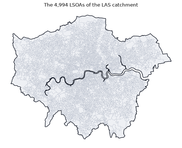
These are the 4,994 LSOAs LAS serves — Greater London’s 5,042 minus the 48 Brentwood LSOAs covered by EEAST. The gap on the Thames is the river itself; ambulances cross it only at bridges, which the travel times (step 2) capture.
The chain does not operate on polygons but on their rook-adjacency
dual graph — one node per LSOA, one edge per pair of LSOAs sharing a
boundary segment. plot_dual_graph draws it:
import json

with open("_static/las_dual_graph_edges.json") as f:
    edges = json.load(f)["edges"]

fp.plot_dual_graph(
    lsoa, edges, id_col="LSOA21CD", boundary=boundary,
    title=f"Rook-adjacency dual graph ({len(edges):,} edges)",
);
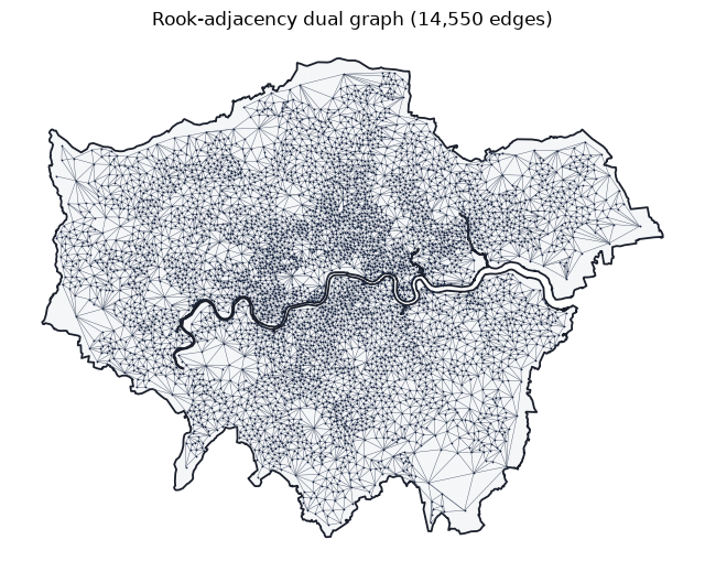
Every district the chain proposes is a connected subgraph of this
graph; each node carries its LSOA’s integer annual demand. Building
this graph from the polygons is exactly what Graph.from_geodataframe
does in step 1 below (plot_dual_graph can also compute the adjacency
itself when you pass no edge list — here we pass the paper’s 14,550
edges, computed from the full-resolution geometry, because the
simplified docs polygons would miss a handful of contacts).
For an interactive overview map (borough boundaries, station markers
with tooltips), see the Leaflet section of
Visualization with FalcomPlot; the LAS repo ships
analysis/run_overview_map.py,
which produces it.
The end-to-end pipeline
Geographic data            Travel times
(shapefile/GeoJSON)        (FalcomTravel)
        │                         │
        ▼                         ▼
   Graph.from_file()      Assignment.travel_times = ...
        │                         │
        └────────────┬────────────┘
                     ▼
        check_facility_density()         ← Assumption 6.1
                     │
              [repair if needed]
                     ▼
       Partition.from_random_assignment()
                     │
                     ▼
              ChainState.initial()
                     │
                     ▼
              MarkovChain(...)
                     │
              [callbacks: ensemble, recorder]
                     ▼
                 .report() / animation
1. Build the graph from your data
Use Graph.from_file for shapefiles / GeoPackages / GeoJSON, or
Graph.from_geodataframe if you already have a GeoDataFrame in
memory. Both accept the same column kwargs.
from falcomchain import Graph

graph = Graph.from_file(
    "districts.shp",
    demand_col="POP",                # column holding demand (population, workload, etc.)
    candidate_col="is_clinic",        # 0/1 column for level-1 candidates
    super_candidate_col="is_hub",     # 0/1 column for level-2 candidates (optional)
    reproject=True,                   # convert lat/lon to UTM for area/perimeter
)
The full reference, including extra columns, CRS handling, and common
errors, lives in Working with GeoDataFrames. The
attribute schema (what demand, candidate, super_candidate mean)
is in Graph Attribute Schema.
2. Compute travel times with FalcomTravel
Travel times feed Assignment.travel_times and drive the level-1
covering radius (Eq. 17) and the optional energy objective
(demand-weighted travel time). For real road networks,
FalcomTravel produces the
matrix from OSM data (multimodal via r5r, or pure-Python via OSMnx):
import falcomtravel as ft
from falcomchain.partition.assignment import Assignment

coords = ft.coords_from_graph(graph, x="C_X", y="C_Y")   # (lon, lat)
backend = ft.R5RBackend(
    data_path="data/london",          # OSM .pbf + GTFS .zip
    coords=coords,
    timezone="Europe/London",
)
matrix = backend.compute(
    origins=station_nodes,
    destinations=list(coords),
    mode=ft.Mode.DRIVE,
)
matrix.to_parquet("travel_times.parquet")     # compute once, reuse

Assignment.travel_times = matrix.as_dict()
The full backend guide — including diagnose() for catching
disconnected road fragments before an hour-long routing run, and the
dependency-free fallbacks for prototyping — is on the
Travel Times with FalcomTravel page.
3. Verify Assumption 6.1
Before running a chain on real data, verify that the candidate set is dense enough that no facility-free region can form a valid district. A real candidate set with sparse coverage will trap the chain.
from falcomchain import check_facility_density, repair_facility_density

report = check_facility_density(graph, demand_target=50_000, epsilon=0.10, c_min=2)
if not report.passes:
    print(f"Adding artificial candidates to repair {len(report.violating_components)} components")
    added = repair_facility_density(
        graph,
        demand_target=50_000,
        epsilon=0.10,
        c_min=2,
        strategy="weighted_center",
    )
    # Each added node now has graph.nodes[n]["candidate_artificial"] = 1
    # so downstream tools (e.g. ensemble analysis) can distinguish synthetic
    # candidates from real ones.
LAS reality check. On the London graph, the 66 real stations do
not fragment the LSOA graph — the candidate-free subgraph remains
one huge connected component, so Assumption 6.1 fails at every
operational (demand_target, c_min) combination and the repair step
is mandatory. At the paper’s calibration the per-component demand cap
is Vol_max = c_min · (1 − ε) · w_unit = 9,254 calls per year, and
repair grows the candidate set to 1,831 sites (66 real stations plus
1,765 artificial — 36.7% of LSOAs). See
analysis/01_feasibility.md
for the full report.
Full details and strategy comparison: Candidate Feasibility.
4. Build the initial partition
from falcomchain import Partition

partition = Partition.from_random_assignment(
    graph=graph,
    epsilon=0.1,
    demand_target=1500,
    assignment_class=None,
    capacity_level=2,
    # super_assignment={node: zone_id}    # if zones are externally given
    # init_super_partition=True,           # paper-faithful initial level-2 partition
    # epsilon_super=0.15,                  # required when init_super_partition=True
)
By default the initial level-2 partition is identity (each level-1
district is its own superdistrict) — cheap, and fine because the
first hierarchical_recom step resamples it anyway. Pass
init_super_partition=True to instead build the initial level-2
partition by recursively partitioning the supergraph (paper Section 5.1
“Initialization”). Useful when you want an honest initial state for
ensemble analysis from step 0.
5. Run the chain
The mechanics are the same as on the demo grid. See Running a FalCom Chain for the full walk-through; the only difference for real data is scale (chains typically run 5,000–50,000 steps) and the optional recording layer for animations.
6. Save and reload chain state
A graph with the partition baked in is a complete description of a chain state — you can serialize it as a single artifact:
import pickle

# Save
partition.write_to_graph()  # writes 'district' attribute on each node
                            # plus 'teams_per_district' and 'capacity_level'
                            # on the graph itself
with open("state.pkl", "wb") as f:
    pickle.dump(graph, f)

# Reload (no need to recompute the partition)
with open("state.pkl", "rb") as f:
    graph = pickle.load(f)
partition = Partition.from_graph(graph)
For the partition alone (not the graph), use
partition.save_json("partition.json") and
Partition.load_json("partition.json", graph).
7. Record for animation
To produce data that the FalcomPlot JS animation app can replay step by step:
from falcomchain.tree.snapshot import Recorder

recorder = Recorder("output/", record_substeps=True)
recorder.write_header(graph, partition, params={
    "epsilon": 0.1,
    "demand_target": 1500,
    "capacity_level": 3,
})

chain = MarkovChain(..., recorder=recorder)
for state in chain:
    pass
recorder.close()

# Export to JSON for the dashboard
Recorder.export_to_json("output/", "output/json/")
The recorder writes a compact binary trajectory (chain.fcrec) plus
optional per-step substep JSON for the four-phase animation.
8. Real-data caveats
Missing
crs— if your shapefile has no CRS, areas and perimeters will be in degrees-squared (almost certainly wrong). Passreproject=Truetofrom_fileor setcrs_override.Disconnected graph — if the graph has multiple connected components (e.g., islands), partition each component separately or use
super_assignmentto keep them in distinct superdistricts.Heavy-demand outlier nodes — if a single node’s demand exceeds
c_max · demand_target · (1 + ε), the algorithm cannot place it inside any admissible district. Either subdivide the unit, raiseepsilon, or merge it with neighbors before building the graph.Travel-time matrix mismatches —
Assignment.travel_timeskeys must matchgraph.nodesexactly. If FalcomTravel uses GEOIDs and your graph is built with sequential integers, build a key map before assignment.
Where to go next
Running a FalCom Chain — full chain mechanics.
Optimization Methods — sampling vs Boltzmann optimization vs custom acceptance.
Ensemble Analysis — boundary, facility, and capacity statistics across samples, including the London Ambulance convergence diagnostics.
Visualization with FalcomPlot — every plotting helper used above.