Running a FalCom Chain

Goal of this page

Understand every knob of a chain run — partition, ChainState, proposal, acceptance — by running a 300-step chain on the shared demo grid and inspecting what it produces.

This page walks through a complete chain run end-to-end. For deeper dives into individual pieces, see:

• Candidate Feasibility — verify and repair the candidate set before running.

• Travel Times — real travel-time matrices with FalcomTravel.

• Level-2 Facilities — opt into level-2 facility assignment.

• Ensemble Analysis — accumulate boundary, facility, and capacity statistics across samples.

1. Load the graph and set travel times

import json
import networkx as nx
from falcomchain.partition.assignment import Assignment

with open("_static/demo_grid_10x10.json") as f:
    data = json.load(f)
graph = nx.node_link_graph(data, edges="links")

# Manhattan-distance travel times. For real graphs, use FalcomTravel
# to compute travel times from OSM/road networks — see the
# "Travel Times with FalcomTravel" page.
Assignment.travel_times = {
    (a, b): float(
        abs(graph.nodes[a]["C_X"] - graph.nodes[b]["C_X"])
        + abs(graph.nodes[a]["C_Y"] - graph.nodes[b]["C_Y"])
    )
    for a in graph.nodes for b in graph.nodes
}

print(f"{graph.number_of_nodes()} nodes, {graph.number_of_edges()} edges")
print(f"travel times set: {len(Assignment.travel_times)} entries")

100 nodes, 180 edges
travel times set: 10000 entries

2. Build the initial partition

from falcomchain import Partition
from falcomchain.random import set_seed

set_seed(42)

# Seed the initial partition on the *achievable* per-team load total / k
# (with k = ceil(total / w) teams), not the raw target w: seeding on w
# starves the last district below the balance window. Capacities stay in
# the safe range c in {1, 2}, where the recursive partitioner provably
# never stalls (see the paper); c >= 3 needs the capacity-block form.
import math
_total = sum(d["demand"] for _, d in graph.nodes(data=True))
seed_demand_target = _total / max(1, math.ceil(_total / 1000))

partition = Partition.from_random_assignment(
    graph=graph,
    epsilon=0.3,
    demand_target=seed_demand_target,
    assignment_class=None,
    capacity_level=2,
)
print(f"{len(partition.parts)} level-1 districts")

5 level-1 districts

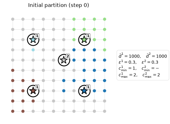
The initial partition has identity level-2 grouping (every level-1 district is its own superdistrict); the first hierarchical_recom step resamples it.

3. Wrap in a ChainState

ChainState is the MCMC view of a partition: it carries the inverse temperature β, hard-feasibility flag, level-1 facility assignment, and (optionally) a level-2 facility assignment.

from falcomchain import SuperFacilityAssignment
from falcomchain.markovchain.state import ChainState

state = ChainState.initial(
    partition=partition,
    energy=0.0,                                                   # placeholder, unused in sampling mode
    beta=1.0,
    super_facility_fn=SuperFacilityAssignment.from_state,         # opt in to level-2
)
print(f"β = {state.beta}")

β = 1.0

Note

No energy function in pure sampling mode. FalCom is a sampler by default — it has no objective. If you also want to optimize an objective (e.g. demand-weighted travel time), pass energy_fn=compute_energy here AND use boltzmann instead of always_accept below. See Optimization Methods for the full story.

4. Configure the chain

from functools import partial
from falcomchain import (
    MarkovChain,
    always_accept,
    hierarchical_recom,
)

proposal = partial(
    hierarchical_recom,
    epsilon_base=0.3,
    epsilon_super=0.3,
    demand_target=1000,
)

chain = MarkovChain(
    proposal=proposal,
    constraints=lambda p: True,  # accept all valid topologies
    accept=always_accept,         # pure sampling
    initial_state=state,
    total_steps=300,
)

Sampling vs optimization

Use case	accept	beta
Sampling from the feasible region (paper default)	always_accept	irrelevant
Boltzmann optimization (find low-energy designs)	boltzmann	small (0.1) – large (5.0+)

Higher β concentrates the chain on lower-energy states. For a typical ensemble run, use always_accept and let β be a no-op; for optimization, use boltzmann with β chosen via annealing. Note that boltzmann is a heuristic optimizer (not a true Metropolis-Hastings sampler) — see Optimization Methods for the full caveats.

5. Run and inspect

We snapshot the full ChainState (not just the Partition) so the plotting helpers can read state.facility.centers for each frame and mark the assigned facility per district.

snapshots = []
for s in chain:
    snapshots.append(s)

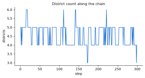
n_districts = [len(s.partition.parts) for s in snapshots]
print(f"steps observed:        {len(snapshots)}")
print(f"district count range:  {min(n_districts)} – {max(n_districts)}")

steps observed:        300
district count range:  3 – 6

Two quick diagnostics tell you whether the run behaved. First, the district count over time — the capacitated proposal is allowed to change it (a merged region can be re-split into a different number of districts), and a healthy chain wanders within a narrow band instead of drifting:

import falcomplot as fp

fig = fp.plot_trace(
    [n_districts], value_label="districts",
    show_legend=False, title="District count along the chain",
)

Second, demand balance: the distribution of demand-per-team across all sampled districts. Note where it centers — when the total demand does not divide evenly by the nominal target w, the proposal recenters each region on the achievable per-team load (total demand over k = ceil(total / w) teams), so the histogram concentrates around that value, slightly below the nominal target, with spread controlled by ε:

import matplotlib.pyplot as plt

per_team = [
    sum(graph.nodes[v]["demand"] for v in nodes) / s.partition.teams[pid]
    for s in snapshots[::10]
    for pid, nodes in s.partition.parts.items()
]

fig, ax = plt.subplots(figsize=(6.5, 3))
ax.axvspan(seed_demand_target * (1 - 0.3), seed_demand_target * (1 + 0.3),
           color="#dfe9f5", label="±ε around achievable load")
ax.hist(per_team, bins=24, color="#33608c")
ax.axvline(seed_demand_target, color="#1d3557", lw=1.4,
           label=f"achievable load ({seed_demand_target:.0f})")
ax.axvline(1000, color="k", lw=1, ls="--", label="nominal target w")
ax.set_xlabel("district demand per team")
ax.set_ylabel("count (every 10th sample)")
ax.legend(fontsize=8)
ax.set_title("Demand balance across sampled districts");

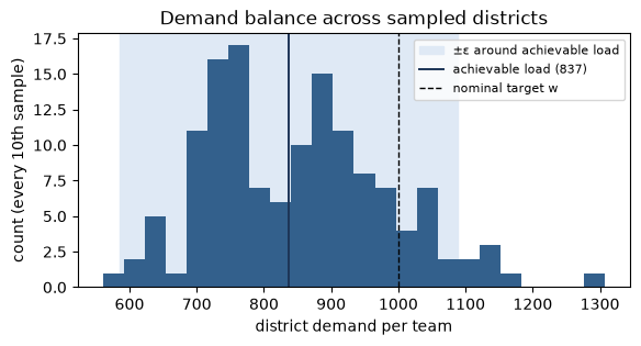
A distribution drifting away from the shaded band — or growing a heavy tail — would mean the balance constraint is being satisfied only via the extremes of the tolerance window, a hint to lower ε or revisit the target.

6. Visualizing initial vs final partition

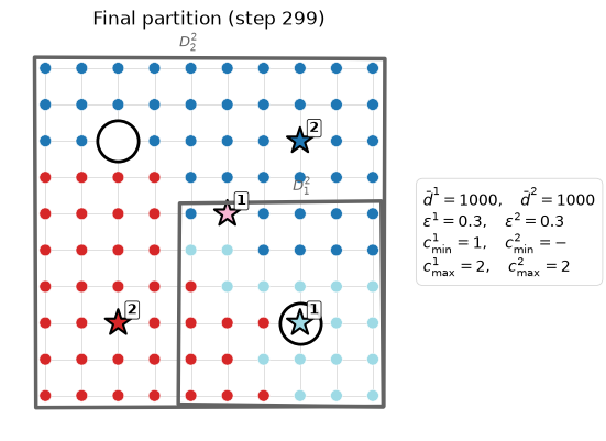
The shared demo grid has 5 high-demand “city centers” (clearly different colors below) and 95 low-demand rural nodes. After the chain runs, every district contains exactly one city — that’s the heterogeneous demand pulling the partition into a stable shape.

District membership is encoded by node color, so we don’t draw level-1 boundary edges (they’d duplicate that information).

The plot has two facility tiers:

• Black-bordered stars mark each level-1 district’s assigned facility — the candidate selected as the district’s minimax facility center. The number next to each star is the district’s team count.

• Larger diamonds mark each level-2 superdistrict’s assigned super-facility. Where superdistricts span multiple level-1 districts, the thick black edges outline the super-district boundary.

The right-hand box shows the partition regime: d̄ = demand_target (paper symbol w), ε = balance tolerance, c_min/c_max = per-district capacity bounds.

from falcomplot import plot_partition

plot_partition(
    graph, snapshots[0],
    title="Initial partition (step 0)",
    demand_target=1000, c_min=1, c_max=2, epsilon=0.3,
    demand_target_super=1000, c_max_super=2, epsilon_super=0.3,
);

plot_partition(
    graph, snapshots[-1],
    title=f"Final partition (step {len(snapshots) - 1})",
    demand_target=1000, c_min=1, c_max=2, epsilon=0.3,
    demand_target_super=1000, c_max_super=2, epsilon_super=0.3,
);

For diagnostic plots that show every candidate site (not just the selected facility per district), pass show_all_candidates=True.

7. Animating the chain

falcomplot.animate_chain builds a matplotlib FuncAnimation over a sequence of partitions or states. Returning the animation from a notebook cell embeds an HTML5 video player.

from IPython.display import HTML
from falcomplot import animate_chain

# Subsample to keep the animation responsive — every 10th snapshot.
# centers_fn pulls per-frame facility centers from each ChainState.
anim = animate_chain(
    graph, snapshots[::10], interval=350,
    centers_fn=lambda state: state.facility.centers,
    super_centers_fn=lambda state: (
        state.super_facility.centers if state.super_facility else None
    ),
    demand_target=1000, c_min=1, c_max=2, epsilon=0.3,
    demand_target_super=1000, c_max_super=2, epsilon_super=0.3,
)
HTML(anim.to_jshtml())

Once Loop Reflect

For the interactive JS animation with spanning-tree details and phase-by-phase replay, attach a Recorder to the chain (see section 8 below) and load the binary trajectory in FalcomPlot’s Vite-based viewer.

8. Common patterns

Recording for animation

Pass a Recorder to capture every step into a binary trajectory file that FalcomPlot’s JS animation app can replay:

from falcomchain.tree.snapshot import Recorder

recorder = Recorder("output/", record_substeps=True)
recorder.write_header(graph, partition, params={"epsilon": 0.3, "demand_target": 500})

chain = MarkovChain(..., recorder=recorder)
for state in chain:
    pass
recorder.close()

Recorder.export_to_json("output/", "output/json/")  # for the dashboard

Ensemble callbacks

Pass EnsembleStats.observe as a callback to accumulate boundary, facility, and capacity statistics during the chain — see Ensemble Analysis.

from falcomchain import EnsembleStats

ensemble = EnsembleStats(burn_in=200, thin=5)
chain = MarkovChain(..., callbacks=[ensemble.observe])
for state in chain:
    pass
report = ensemble.report()

Pluggable extension points

Component	How to swap	Default
Spanning-tree sampler	bipartition_tree(tree_sampler=...)	Wilson’s uniform
Candidate-awareness ψ	CutParams(psi_fn=...)	phi · exp(-γ · r)
Energy function (objective, opt-in)	ChainState.initial(energy_fn=...)	None — sampler mode; pass compute_energy for the optimizer
Acceptance rule	MarkovChain(accept=...)	always_accept
Distance metric	Assignment.travel_times	None
Level-2 facility selector	SuperFacilityAssignment.from_state(selection_fn=...)	minimax_super_selector
Upper-level partitioner	hierarchical_recom(super_partitioner=...)	resample_super_partition

Every algorithmic choice is configurable so you can test the paper’s future-work variants without forking the library.

9. Where to go next

• Verify your candidate set before running on real data — Candidate Feasibility.

• Set up level-2 facility analysis for hierarchical questions — Level-2 Facilities.

• Aggregate across samples to find robust boundaries and essential facilities — Ensemble Analysis.

• See every plotting helper used above in one place — Visualization with FalcomPlot.