Getting Started
Goal of this page
Install FalcomChain and run a complete chain — graph, travel times, partition, 100 MCMC steps, and a first plot — in five minutes.
Installation
pip install "falcomchain @ git+https://github.com/kirtisoglu/FalcomChain.git@main"
Requires Python 3.12+. For the plots below, also install the companion plotting library:
pip install "falcomplot @ git+https://github.com/kirtisoglu/FalcomPlot.git@main"
The big picture
A FalcomChain workflow has four steps:
Build a
Graphfrom your geographic data — each node needs ademandand a 0/1candidateflag (schema).Set travel times — a
(origin, destination) -> secondsdict (Travel Times).Run a
MarkovChain— each step proposes a new feasible plan.Analyze the ensemble — robust boundaries, essential facilities (Ensemble Analysis).
The code below is fully self-contained and executed at build time — you can paste it into a fresh notebook and it will run.
1. Build a graph
Real workflows start from a shapefile via Graph.from_file(...)
(see Working with GeoDataFrames). For a first chain,
the built-in Grid generates a synthetic instance with demand and
candidate attributes already in place:
from falcomchain.graph.grid import Grid
from falcomchain.random import set_seed

set_seed(2025)
graph = Grid(dimensions=(10, 10), num_candidates=30, density="random").graph

sample = next(iter(graph.nodes))
print(f"{graph.number_of_nodes()} nodes; node {sample}: {graph.nodes[sample]}")
100 nodes; node (0, 0): {'demand': 50, 'C_X': 0, 'C_Y': 0, 'area': 1, 'candidate': True, 'super_candidate': 0, 'boundary_node': True, 'boundary_perim': 2}
2. Set travel times
Facility assignment picks each district’s center by minimizing the worst travel time to any node in the district, so the chain needs a distance metric. Manhattan distance is fine for a grid; for real road networks use FalcomTravel.
from falcomchain.partition.assignment import Assignment

Assignment.travel_times = {
    (a, b): float(
        abs(graph.nodes[a]["C_X"] - graph.nodes[b]["C_X"])
        + abs(graph.nodes[a]["C_Y"] - graph.nodes[b]["C_Y"])
    )
    for a in graph.nodes for b in graph.nodes
}
print(f"{len(Assignment.travel_times)} OD pairs set")
10000 OD pairs set
3. Initial partition and chain
Partition.from_random_assignment builds a feasible starting plan:
contiguous districts, each within the demand-balance window and each
containing at least one candidate. Wrapping it in a ChainState adds
the facility assignment.
import math
from functools import partial

from falcomchain import (
    MarkovChain,
    Partition,
    always_accept,
    hierarchical_recom,
)
from falcomchain.markovchain.state import ChainState

# Seed the initial recursion on the achievable per-team load (total / k
# with k = ceil(total / target)) so the last district stays in balance.
demand_target = 1000
total = sum(d["demand"] for _, d in graph.nodes(data=True))
seed_target = total / max(1, math.ceil(total / demand_target))

partition = Partition.from_random_assignment(
    graph=graph,
    epsilon=0.3,             # demand-balance tolerance
    demand_target=seed_target,
    assignment_class=None,
    capacity_level=2,        # up to 2 teams per district
)
state = ChainState.initial(partition=partition, energy=0.0, beta=1.0)

chain = MarkovChain(
    proposal=partial(hierarchical_recom, epsilon_base=0.3,
                     epsilon_super=0.3, demand_target=demand_target),
    constraints=lambda p: True,
    accept=always_accept,     # pure sampling — FalCom's default mode
    initial_state=state,
    total_steps=100,
)

snapshots = list(chain)
print(f"{len(snapshots)} states sampled; "
      f"{len(snapshots[-1].partition.parts)} districts in the final plan")
100 states sampled; 5 districts in the final plan
4. Look at what you sampled
from falcomplot import plot_partition

plot_partition(
    graph, snapshots[-1],
    title="A sampled plan (step 100)",
    demand_target=demand_target, c_min=1, c_max=2, epsilon=0.3,
);
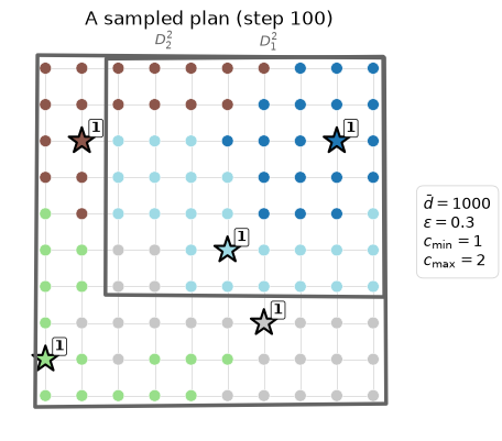
Node colors are districts; each black-bordered star is that district’s facility center, with the district’s team count next to it.
One plan is a starting point — the value of MCMC is the ensemble. Run
longer chains and aggregate with
EnsembleStats, then render boundary-frequency maps
with FalcomPlot.
Where to go next
Algorithm Overview — what the chain actually does at each step, and why MCMC.
Working with GeoDataFrames — build the graph from your own shapefile.
Travel Times with FalcomTravel — real road-network travel times.
Running a FalCom Chain — every knob of the chain, explained on the shared demo grid.
Quickstart tutorial — the same material as a downloadable notebook.