Ensemble Analysis

Goal of this page

Turn a chain’s samples into decisions: accumulate boundary, facility, and capacity statistics with EnsembleStats, check convergence, and read the resulting maps.

FalCom is the first MCMC sampler for facility location. The ensemble module turns that sampler into a decision-support tool by analyzing the distribution of near-optimal designs, not just a single optimum.

What it measures

For each sample drawn from the chain, the module accumulates:

• Boundary frequency — how often each edge is a district boundary. High = robust boundary, low = fragile.

• Facility stability — how often each candidate is selected as a facility center. High = essential, low = substitutable.

• Capacity utilization — per-sample coefficient of variation of demand-per-team and covering-radius statistics, accumulated with Welford’s online algorithm.

A small grid example

We load the shared 10×10 demo grid (the same dataset used by the Candidate Feasibility and Level-2 Facilities pages). The grid has heterogeneous demand: 5 “city center” nodes with high demand (700), 95 “rural” nodes with low demand (16). Heterogeneity is what makes ensemble analysis informative — without it, every partition is exchangeable under the grid’s symmetries and no boundary is meaningfully more robust than another.

We then run a real hierarchical_recom chain for 400 steps, discarding the first 40 (burn-in) and recording every other step (thinning) — 180 samples in total.

import json
from functools import partial

import networkx as nx

from falcomchain import (
    EnsembleStats,
    MarkovChain,
    Partition,
    always_accept,
    hierarchical_recom,
)
from falcomchain.markovchain.state import ChainState
from falcomchain.partition.assignment import Assignment
from falcomchain.random import set_seed

with open("_static/demo_grid_10x10.json") as f:
    graph = nx.node_link_graph(json.load(f), edges="links")

# Manhattan-distance travel times keep the example tiny.
Assignment.travel_times = {
    (a, b): float(
        abs(graph.nodes[a]["C_X"] - graph.nodes[b]["C_X"])
        + abs(graph.nodes[a]["C_Y"] - graph.nodes[b]["C_Y"])
    )
    for a in graph.nodes for b in graph.nodes
}

set_seed(42)

# Seed the initial partition on the *achievable* per-team workload.
# With total demand D and a workload cap of w per team, the coverage
# rule needs k = ceil(D / w) teams, so the k districts must average
# D / k, which is strictly below the nominal w. Centering the initial
# recursion on D / k (rather than on w) keeps the last district inside
# the balance window; this mirrors the recentering the chain proposal
# does locally. Capacities are kept in the safe range c in {1, 2}, where
# the recursive partitioner provably never stalls (see the paper); c >= 3
# needs the capacity-block reparametrization.
import math

demand_target = 1000
total_demand = sum(d["demand"] for _, d in graph.nodes(data=True))
k_teams = max(1, math.ceil(total_demand / demand_target))
seed_demand_target = total_demand / k_teams

partition = Partition.from_random_assignment(
    graph=graph,
    epsilon=0.3,
    demand_target=seed_demand_target,
    assignment_class=None,
    capacity_level=2,
)
state = ChainState.initial(partition=partition, energy=0.0, beta=1.0)

ensemble = EnsembleStats(burn_in=40, thin=2)
chain = MarkovChain(
    proposal=partial(
        hierarchical_recom,
        epsilon_base=0.3,
        epsilon_super=0.3,
        demand_target=1000,
    ),
    constraints=lambda p: True,
    accept=always_accept,
    initial_state=state,
    total_steps=400,
    callbacks=[ensemble.observe],
)
list(chain)

ensemble.n_samples

180

Inspecting boundary frequency

boundary_freq = ensemble.boundary.frequencies()
print(f"Edges that ever appeared as boundaries: {len(boundary_freq)}")
print(f"Robust  (>=70% of samples): {len(ensemble.boundary.robust(0.7))}")
print(f"Fragile (<50% of samples):  {len(ensemble.boundary.fragile(0.5))}")

Edges that ever appeared as boundaries: 179
Robust  (>=70% of samples): 0
Fragile (<50% of samples):  175

Boundary heatmap

falcomplot ships the boundary-frequency map as a single call, so we do not hand-roll the drawing. Import it as fp and pass the edge list, the per-edge frequencies, and the node positions. Edges are colored by how often they serve as a district boundary: dark = robust (nearly always a boundary), pale = fragile.

import falcomplot as fp

pos = {n: (d["C_X"], d["C_Y"]) for n, d in graph.nodes(data=True)}
edges = [(min(u, v), max(u, v)) for u, v in graph.edges()]
freqs = [boundary_freq.get(e, 0.0) for e in edges]

fig = fp.plot_boundary_frequency(
    edges, freqs, pos,
    aspect="equal", floor=0.0,
    colorbar_label="boundary frequency",
    title="Boundary frequency map (demo grid)",
)

Matplotlib is building the font cache; this may take a moment.

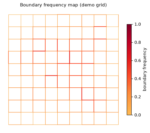
The robust boundaries (dark) tend to lie between cities — these are the cuts the chain makes consistently, regardless of starting state. Boundaries within rural regions remain pale because the chain has many equally good ways to draw them.

Inspecting facility stability

facility_freq = ensemble.facility.frequencies()
print(f"Candidates ever selected: {len(facility_freq)}")
print(f"Essential (>=90%):        {len(ensemble.facility.essential(0.9))}")
print(f"Substitutable (<50%):     {len(ensemble.facility.substitutable(0.5))}")

Candidates ever selected: 9
Essential (>=90%):        3
Substitutable (<50%):     4

Selection rates read best as a chart — essential candidates (selected in nearly every sample) stand apart from the substitutable tail:

import matplotlib.pyplot as plt

ranked = sorted(facility_freq.items(), key=lambda kv: -kv[1])
nodes = [str(n) for n, _ in ranked]
rates = [f for _, f in ranked]

fig, ax = plt.subplots(figsize=(7, 3))
colors = ["#b3452c" if r >= 0.9 else "#33608c" if r >= 0.5 else "#a9bfd6"
          for r in rates]
ax.bar(range(len(nodes)), rates, color=colors)
ax.axhline(0.9, color="#b3452c", lw=0.8, ls="--")
ax.axhline(0.5, color="#a9bfd6", lw=0.8, ls="--")
ax.set_xticks(range(len(nodes)), nodes, rotation=90, fontsize=7)
ax.set_ylabel("selection frequency")
ax.set_title("Facility stability: essential (red) vs substitutable (pale)");

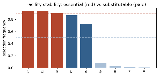
Candidates above the 0.9 line are essential — the chain picks them in nearly every sampled plan, so removing them would degrade most good designs. Candidates below 0.5 are substitutable: other sites cover their role.

Capacity utilization summary

Per-sample CV of demand-per-team and covering-radius statistics across the ensemble:

ensemble.capacity.summary()

{'demand_cv': {'n': 180,
  'mean': 0.14652340353869048,
  'std': 0.044994433096869374,
  'min': 0.05323299160813053,
  'max': 0.2711152972252844},
 'max_radius': {'n': 180,
  'mean': 4771.71111111111,
  'std': 1454.3866087451036,
  'min': 1616.0,
  'max': 9240.0},
 'mean_radius': {'n': 180,
  'mean': 1914.2570370370368,
  'std': 672.5530653261229,
  'min': 838.4,
  'max': 4541.333333333333}}

Full report

report() returns everything in one dict:

report = ensemble.report()
sorted(report.keys())

['boundary_frequencies',
 'capacity',
 'essential_facilities',
 'facility_frequencies',
 'fragile_boundaries',
 'n_samples',
 'robust_boundaries',
 'substitutable_facilities',
 'super_facility_frequencies']

print(f"n_samples:                {report['n_samples']}")
print(f"essential_facilities:     {len(report['essential_facilities'])}")
print(f"substitutable_facilities: {len(report['substitutable_facilities'])}")
print(f"robust_boundaries:        {len(report['robust_boundaries'])}")
print(f"fragile_boundaries:       {len(report['fragile_boundaries'])}")

n_samples:                180
essential_facilities:     3
substitutable_facilities: 4
robust_boundaries:        0
fragile_boundaries:       175

Burn-in, thinning, and the callback hook

The chain example above already uses the standard MCMC accumulation pattern: EnsembleStats(burn_in=40, thin=2) was passed as a callback to MarkovChain, so the chain feeds every state into ensemble.observe as it runs. Out of 400 chain steps, the first 40 are discarded (burn-in) and only every other remaining step is recorded (thinning), giving n_samples = 180.

For longer chains, raise the burn-in and thinning to match — typical real-world settings are burn_in=500-2000 and thin=10 for chains of 10,000+ steps:

ensemble = EnsembleStats(burn_in=500, thin=10)
chain = MarkovChain(..., total_steps=10_000, callbacks=[ensemble.observe])
list(chain)
report = ensemble.report()

Filtering out artificial candidates

If you ran repair_facility_density before the chain, the ensemble counts artificial candidates alongside real ones. To report only real essential facilities:

real_essential = {
    n: f for n, f in report["essential_facilities"].items()
    if not graph.nodes[n].get("candidate_artificial", 0)
}

A high frequency on an artificial candidate is informative — it means the chain wants a facility there — but should not be presented as “essential” without that context.

Convergence diagnostics with FalcomPlot

The ensemble statistics above are only meaningful once the chain has reached its stationary regime. Because tight mixing-time bounds are not known for recombination-style chains, convergence is assessed empirically from several independently seeded chains, using two diagnostics that falcomplot computes directly: the Gelman–Rubin potential scale reduction factor $\hat R$ (do the chains agree?) and the effective sample size (how many independent draws does a correlated run provide?).

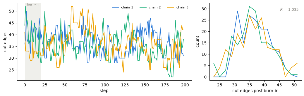
Record a scalar summary along each chain — here the number of cut (boundary) edges, though the energy or a district count works just as well — then hand the list of traces to falcomplot. We run three independently seeded chains on the same demo grid:

import falcomplot as fp

def run_chain(seed, steps=200):
    set_seed(seed)
    partition = Partition.from_random_assignment(
        graph=graph, epsilon=0.3, demand_target=seed_demand_target,
        assignment_class=None, capacity_level=2)
    state = ChainState.initial(partition=partition, energy=0.0, beta=1.0)
    trace = []
    def record(st, accepted):
        m = st.partition.assignment.mapping
        trace.append(sum(1 for u, v in graph.edges() if m[u] != m[v]))
    chain = MarkovChain(
        proposal=partial(hierarchical_recom, epsilon_base=0.3,
                         epsilon_super=0.3, demand_target=demand_target),
        constraints=lambda p: True, accept=always_accept,
        initial_state=state, total_steps=steps, callbacks=[record])
    list(chain)
    return trace

burn_in = 20
traces = [run_chain(seed) for seed in (1, 2, 3)]

rhat = fp.gelman_rubin([t[burn_in:] for t in traces])
ess  = sum(fp.effective_sample_size(t[burn_in:]) for t in traces)
print(f"R-hat = {rhat:.3f}   ESS = {ess:.0f}")

R-hat = 1.035   ESS = 59

plot_convergence returns a two-panel figure: the left panel overlays the chains’ traces with the burn-in shaded, and the right panel shows their post-burn-in distributions with the split $\hat R$ annotated:

fig = fp.plot_convergence(
    traces, burn_in=burn_in, value_label="cut edges",
    labels=[f"chain {i}" for i in (1, 2, 3)],
)

A single-chain trace is drawn with fp.plot_trace, and a boundary-frequency map over a real dual graph with fp.plot_boundary_frequency, exactly as above.

In the FalCom paper: the London Ambulance Service ensemble

These are the diagnostics behind the case study in the FalCom paper. On the London Ambulance Service instance (a 4,994-node LSOA dual graph with 66 stations across 5 sectors), four independently seeded chains of 10,000 steps were run at the locked capacity-block calibration. fp.plot_convergence on the access-cost trace gives $\hat R \approx 1.00$, and the four chains’ post-burn-in energy distributions coincide:

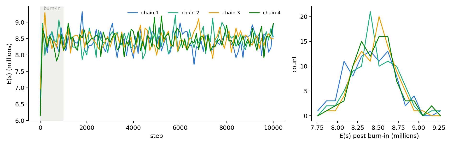
Energy traces of four London Ambulance chains (left, burn-in shaded) and their post-burn-in distributions (right), rendered by fp.plot_convergence. The split Gelman–Rubin statistic is $\hat R \approx 1.00$.

Aggregating the post-burn-in snapshots into a boundary-frequency map with fp.plot_boundary_frequency shows which service-zone boundaries the ensemble fixes and which stay contested:

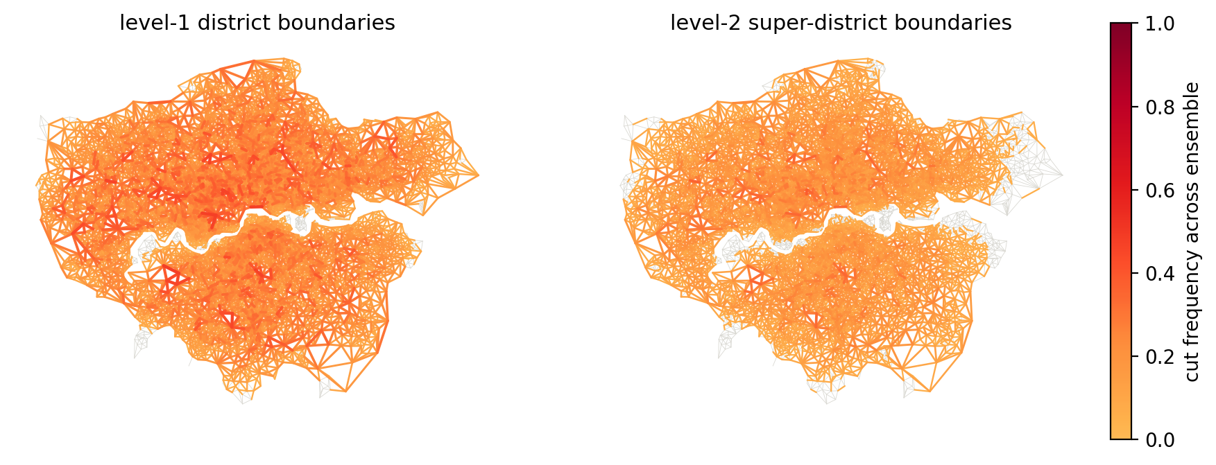
Level-1 district and level-2 super-district boundary frequencies across the London Ambulance ensemble, rendered by fp.plot_boundary_frequency.

The current operational layout lands within 4.6% of the best matched-count configuration the search found. See the FalCom paper for the full setup and metrics.

API reference

EnsembleStats(burn_in=0, thin=1)

Main coordinator. Holds boundary, facility, and capacity analyzers.

• observe(state, accepted) — record one step

• report() — return summary dict

• n_samples — number of recorded samples

BoundaryCounter()

• observe(state, accepted)

• frequencies() — dict[edge, float]

• robust(threshold=0.9) — edges above threshold

• fragile(threshold=0.5) — edges below threshold

FacilityCounter()

• observe(state, accepted)

• frequencies() — dict[node, float] (level-1)

• super_frequencies() — dict[node, float] (level-2)

• essential(threshold=0.9) — nodes above threshold

• substitutable(threshold=0.5) — nodes below threshold

CapacityStats()

• observe(state, accepted)

• summary() — dict with demand_cv, max_radius, mean_radius (each a Welford summary)

• demand_cv, max_radius, mean_radius — WelfordStats instances

WelfordStats()

Online mean/variance via Welford’s algorithm.

• update(x) — add observation

• mean, variance, std, min, max, n — properties

• summary() — dict with all stats