Candidate Feasibility

Goal of this page

Verify that your candidate set satisfies Assumption 6.1 before running a chain, and repair it with artificial candidates when it does not — including how to choose among the six placement strategies.

The FalCom chain converges to a unique stationary distribution only when the candidate set is dense enough that no facility-free region of the graph can form a valid district on its own. This page shows how to verify the condition (Assumption 6.1 in the paper) and how to add artificial candidates if it fails.

The condition

For a graph G with per-team workload w (= demand_target), tolerance ε, and minimum district capacity c_min, every connected component of the facility-free subgraph G[V \ F] must satisfy:

$$ d_C ;<; (1 - \varepsilon) \cdot c_{\min} \cdot w $$

If a connected facility-free region carries demand at or above this threshold, the chain can construct a valid district (of the smallest allowed capacity) that contains no facility — a state from which it cannot make progress. Verification is O(|V| + |E|) via a single BFS.

Note

The paper states the condition with c_min = 1 (the chain may propose capacity-1 districts). This library generalizes: pass c_min=2 (or higher) to opt into a stricter algorithm. The threshold then scales linearly, so far fewer candidates are needed. The trade-off: the chain explores a smaller state space (no single-team districts).

The example dataset

We use a 10×10 grid (100 nodes, 180 edges) with about 30 candidate facilities placed by a weighted-center seeding pass plus a small random perturbation (so Assumption 6.1 fails by just a few candidates, giving the repair routine something visible to fix). Every node has demand 50. Download demo_grid_10x10.json and use it for any of FalcomChain’s modules.

import json
import networkx as nx

with open("_static/demo_grid_10x10.json") as f:
    data = json.load(f)

graph = nx.node_link_graph(data, edges="links")
n_cands = sum(1 for n, d in graph.nodes(data=True) if d["candidate"])
print(f"{graph.number_of_nodes()} nodes, {graph.number_of_edges()} edges, "
      f"{n_cands} candidates")

100 nodes, 180 edges, 10 candidates

Visualizing the initial state

Visualization helpers live in FalcomPlot, the companion plotting library. :func:falcomplot.plot_grid reads the same node attributes (C_X, C_Y, candidate, super_candidate) and covers all the docs use cases — candidate display, partition coloring, artificial-candidate highlights, level-2 facility rings.

from falcomplot import plot_grid

plot_grid(
    graph,
    title="10x10 grid — initial candidate placement",
    show_level2_candidates=False,  # this page is about level-1 only
);

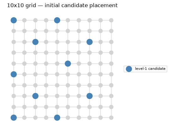
The candidates cover most of the grid; whether the remaining facility-free region satisfies the assumption depends on the specific demand_target and epsilon you choose.

Checking the assumption

from falcomchain import check_facility_density

report = check_facility_density(graph, demand_target=1000, epsilon=0.1)
report

<FeasibilityReport FAILS: 1 violating components, worst demand=1440.00, threshold=900.00>

The threshold is (1 - 0.1) · 1000 = 900, but at least one facility-free component carries demand above the threshold — a violation:

print(f"passes:        {report.passes}")
print(f"threshold:     {report.threshold}")
print(f"violating:     {len(report.violating_components)} component(s)")
print(f"worst demand:  {report.worst_demand}")

passes:        False
threshold:     900.0
violating:     1 component(s)
worst demand:  1440

Repairing the violation

repair_facility_density adds artificial candidates until the assumption holds. The default strategy is "weighted_center" — the demand-weighted graph 1-center of each violating component.

from falcomchain import repair_facility_density

added = repair_facility_density(
    graph,
    demand_target=1000,
    epsilon=0.1,
    strategy="weighted_center",
)
print(f"Added {len(added)} artificial candidates")

Added 11 artificial candidates

Re-checking confirms the assumption now holds:

report_after = check_facility_density(graph, demand_target=1000, epsilon=0.1)
report_after

<FeasibilityReport passes (threshold=900.00)>

Visualizing the repaired grid

Artificial candidates appear as orange squares. Each is positioned at the center of a violating region the original candidate set failed to cover.

plot_grid(
    graph,
    title="After repair — artificial candidates added",
    artificial_candidates=added,
    show_level2_candidates=False,
);

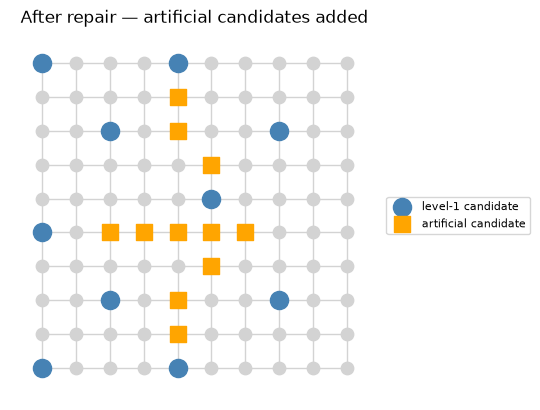
Every added node carries candidate_artificial = 1, so downstream tools (e.g. the ensemble facility analysis) can distinguish synthetic from real facilities:

sample = next(iter(added))
dict(graph.nodes[sample])

{'demand': 16,
 'C_X': 6,
 'C_Y': 4,
 'area': 1,
 'candidate': 1,
 'boundary_node': 0,
 'boundary_perim': 0,
 'super_candidate': 0,
 'candidate_artificial': 1}

Comparing the placement strategies

repair_facility_density ships six placement strategies. The same violating grid, repaired each way — we reload a fresh copy each time so the strategies don’t see each other’s additions. (metis_separator requires the optional pymetis dependency, so we skip it gracefully when absent.)

def fresh_graph():
    with open("_static/demo_grid_10x10.json") as f:
        return nx.node_link_graph(json.load(f), edges="links")

strategies = (
    "highest_demand", "center", "weighted_center",
    "fast_center", "balanced_separator", "metis_separator",
)

results = {}
for strategy in strategies:
    try:
        g = fresh_graph()
        added_s = repair_facility_density(
            g, demand_target=1000, epsilon=0.1, strategy=strategy
        )
        results[strategy] = len(added_s)
    except ImportError:
        print(f"{strategy}: skipped (optional dependency not installed)")

results

metis_separator: skipped (optional dependency not installed)

{'highest_demand': 34,
 'center': 11,
 'weighted_center': 11,
 'fast_center': 7,
 'balanced_separator': 9}

import matplotlib.pyplot as plt

fig, ax = plt.subplots(figsize=(7, 3))
names = list(results)
ax.barh(names, [results[n] for n in names], color="#33608c")
ax.set_xlabel("artificial candidates added (fewer is better)")
ax.set_title("Repair cost by placement strategy")
ax.invert_yaxis()
for i, n in enumerate(names):
    ax.text(results[n] + 0.05, i, str(results[n]), va="center", fontsize=9)

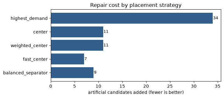
The center-based strategies typically need fewer or as-few candidates, because removing a graph center fragments the violating component more aggressively. With near-uniform demand, highest_demand falls back to an arbitrary tiebreaker and can perform worse. Separator strategies shine on large heterogeneous-demand graphs, where they produce the smallest scaffolds.

When to use which

Situation	Strategy
You want exactly the paper’s procedure	highest_demand
Large graph (>10⁵ nodes), repair speed matters	highest_demand or fast_center
Default real-world case	weighted_center
You don’t trust the demand attribute	center
Very large graph, no external deps	balanced_separator
Heterogeneous demand, smallest scaffold	metis_separator (needs pymetis)

API reference

FeasibilityReport

• passes: bool — True iff the assumption holds.

• threshold: float — (1 − ε) · demand_target.

• violating_components: list[set[node]] — nodes per violating component.

• component_demands: list[float] — demand of each violating component.

• worst_demand: float — max component demand observed.

check_facility_density(graph, demand_target, epsilon=0.1, ...)

Returns a FeasibilityReport. Read-only.

repair_facility_density(graph, demand_target, epsilon=0.1, strategy="weighted_center", ...)

Modifies graph in place. Returns the set of added nodes.

Optional kwargs:

• candidate_attr — node attribute used to mark candidates (default "candidate").

• demand_attr — node attribute holding demand (default "demand").

• artificial_attr — node attribute used to flag added candidates (default "candidate_artificial").

• max_iterations — safety cap (default len(graph.nodes) + 1).