Optimization Methods

Goal of this page

Turn the sampler into an optimizer when you need one low-energy plan: energy functions, Boltzmann acceptance, annealing schedules, and custom acceptance rules — with the caveats spelled out.

FalCom is a sampler by default. Section 3 of the paper deliberately omits an objective — the chain explores the feasible region weighted by the candidate-awareness score ψ, and analysis happens via ensemble statistics. This page is for the opt-in optimizer: an acceptance rule, an inverse temperature β, and an objective function.

Mode	accept	energy_fn	beta	When
Pure sampling (paper default)	always_accept	not set	irrelevant	Build an ensemble; analyze robust boundaries.
Boltzmann optimization	boltzmann	required	small (0.1) – large (5.0+)	Find low-energy designs; simulated-annealing schedule.

The objective function

The optimizer needs an explicit objective. Two pieces wire it up:

1. Pass energy_fn=... to ChainState.initial(...). The state then computes energy_fn(state) once initially and on every state.next() call.

2. Use accept=boltzmann on the MarkovChain. boltzmann reads state.energy and accepts with probability exp(-β · ΔE).

If you set one without the other, things go wrong loudly:

• accept=boltzmann with no energy_fn → RuntimeError on the first proposal. (We refuse to silently degrade to always_accept.)

• energy_fn set with accept=always_accept → energy is computed on every step but never used. Wasteful, not incorrect.

Default energy: compute_energy (demand-weighted travel time)

The library ships compute_energy as a default objective:

E(s) = Σ_D Σ_{v ∈ D} d_v · dist(v, f(D))

For each level-1 district D, the inner sum is the demand-weighted travel time from each base node to the district’s facility center. This penalizes districts where high-demand nodes are far from their facility. To use it, pass it as energy_fn:

from falcomchain.markovchain.energy import compute_energy

state = ChainState.initial(
    ..., energy_fn=compute_energy,
)

compute_energy requires Assignment.travel_times to be set.

Custom objectives

energy_fn is just a callable (ChainState) -> float. Some useful shapes:

• Equity-weighted travel time: Σ_D Σ_v w_v · d_v · dist(...) where w_v upweights vulnerable populations.

• Maximum covering radius: max_D r(D) — minimax over districts.

• Compactness: Polsby-Popper or convex-hull deviation.

• Mixed: weighted sum of any of the above.

def equity_energy(state):
    total = 0.0
    for part_id, nodes in state.parts.items():
        center = state.facility.centers[part_id]
        for v in nodes:
            d = state.assignment.travel_times[(center, v)]
            w = state.graph.nodes[v].get("vulnerability", 1.0)
            demand = state.graph.nodes[v]["demand"]
            total += w * demand * d
    return total

state = ChainState.initial(..., energy_fn=equity_energy)

Important

boltzmann is a heuristic optimizer, not a true Metropolis-Hastings sampler. It omits the proposal-density ratio q(s|s')/q(s'|s) because that ratio is intractable for FalCom (paper Section 6.3, #P-hard per Jerrum & Sinclair). The chain is biased toward low-energy states but does not sample from a Boltzmann distribution. For sampling with convergence guarantees, use always_accept and don’t set energy_fn at all.

Note

Avoid stacking ψ-bias and Boltzmann together unless you mean to. The candidate-awareness score ψ (controlled by gamma and gamma_super) biases the proposal toward small-radius districts. Boltzmann acceptance biases toward low-energy. These are correlated but distinct objectives. For unconfounded energy minimization, use boltzmann with gamma=0 and gamma_super=0. For multi-criterion optimization (small radius and low energy), keep gamma>0 and accept that the chain is optimizing an implicit hybrid.

Setup

import json
import networkx as nx

from falcomchain import (
    MarkovChain,
    Partition,
    always_accept,
    hierarchical_recom,
)
from falcomchain.markovchain.accept import boltzmann
from falcomchain.markovchain.energy import compute_energy
from falcomchain.markovchain.state import ChainState
from falcomchain.partition.assignment import Assignment
from falcomchain.random import set_seed

with open("_static/demo_grid_10x10.json") as f:
    graph = nx.node_link_graph(json.load(f), edges="links")

Assignment.travel_times = {
    (a, b): float(
        abs(graph.nodes[a]["C_X"] - graph.nodes[b]["C_X"])
        + abs(graph.nodes[a]["C_Y"] - graph.nodes[b]["C_Y"])
    )
    for a in graph.nodes for b in graph.nodes
}


def fresh_state(beta, energy_fn=None):
    set_seed(42)
    # Seed on the achievable per-team load total / k, not the raw target;
    # keep capacities in the safe range c in {1, 2}.
    import math
    total = sum(d["demand"] for _, d in graph.nodes(data=True))
    seed_dt = total / max(1, math.ceil(total / 1000))
    partition = Partition.from_random_assignment(
        graph=graph, epsilon=0.3, demand_target=seed_dt,
        assignment_class=None, capacity_level=2,
    )
    return ChainState.initial(
        partition=partition,
        energy=0.0,
        beta=beta,
        energy_fn=energy_fn,
    )

Mode 1: Pure sampling (no objective)

always_accept accepts every feasible proposal. The chain explores the feasible region without computing or considering an objective. Use this to build an ensemble for analysis.

from functools import partial

set_seed(7)
chain = MarkovChain(
    proposal=partial(hierarchical_recom, epsilon_base=0.3, epsilon_super=0.3, demand_target=1000),
    constraints=lambda p: True,
    accept=always_accept,
    initial_state=fresh_state(beta=0.0),  # no energy_fn — no objective
    total_steps=200,
)
n_samples = sum(1 for _ in chain)
print(f"sampling produced {n_samples} states (no energy computed)")

sampling produced 200 states (no energy computed)

The chain visits the feasible region; analyze the resulting samples via Ensemble Analysis. No energy was computed at any step — that’s the point of sampling mode.

Mode 2: Boltzmann optimization

boltzmann accepts the proposal with probability

α = min(1, R(s') · exp(-β · (E(s') - E(s))))

R(s') is the hard feasibility indicator (state.feasible); the exponential is the Boltzmann weight on the energy delta.

At small β the acceptance behaves nearly like sampling but with a mild bias toward lower energy. At large β it becomes near-greedy.

set_seed(7)
chain = MarkovChain(
    proposal=partial(hierarchical_recom, epsilon_base=0.3, epsilon_super=0.3, demand_target=1000),
    constraints=lambda p: True,
    accept=boltzmann,
    initial_state=fresh_state(beta=0.1, energy_fn=compute_energy),
    total_steps=200,
)
soft_energies = [s.energy for s in chain]
print(f"Boltzmann (β=0.1): min={min(soft_energies):.0f}, "
      f"final={soft_energies[-1]:.0f}")

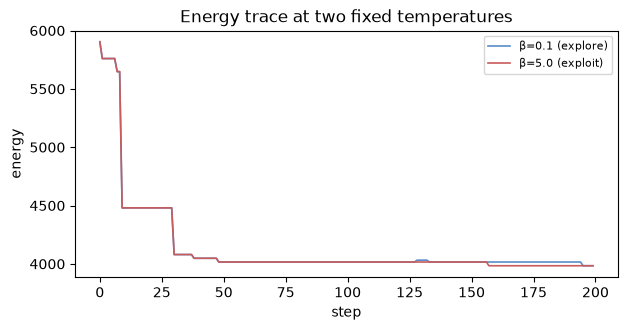
Boltzmann (β=0.1): min=3984, final=3984

For greedy optimization, set β large and run for a long horizon. The simplest schedule is a fixed β; for harder problems, anneal β upward over time.

set_seed(7)
chain = MarkovChain(
    proposal=partial(hierarchical_recom, epsilon_base=0.3, epsilon_super=0.3, demand_target=1000),
    constraints=lambda p: True,
    accept=boltzmann,
    initial_state=fresh_state(beta=5.0, energy_fn=compute_energy),
    total_steps=200,
)
opt_energies = [s.energy for s in chain]
print(f"Boltzmann (β=5.0): min={min(opt_energies):.0f}, "
      f"final={opt_energies[-1]:.0f}")

Boltzmann (β=5.0): min=3984, final=3984

Compare the two β values. The low-temperature chain (β=5.0) locks into low-energy plans quickly but explores little; the high-temperature chain (β=0.1) keeps moving and only drifts downward:

import matplotlib.pyplot as plt

fig, ax = plt.subplots(figsize=(7, 3.2))
ax.plot(soft_energies, label="β=0.1 (explore)", color="#5b8cc8", lw=1.2)
ax.plot(opt_energies,  label="β=5.0 (exploit)", color="#c85b5b", lw=1.2)
ax.set_xlabel("step")
ax.set_ylabel("energy")
ax.legend(fontsize=8)
ax.set_title("Energy trace at two fixed temperatures");

Matplotlib is building the font cache; this may take a moment.

(Pure sampling is omitted from the plot — it computes no energy by design.)

Annealing schedules

A constant β is rarely optimal for hard problems. Annealing — start at small β (broad exploration) and ramp up (greedy refinement) — usually beats a fixed β. The simplest pattern: update state.beta between steps, since it’s a regular attribute.

import math

def temperature(step, total):
    """Geometric annealing from beta=0.1 to beta=5."""
    return 0.1 * math.exp(math.log(50) * step / total)

set_seed(7)
total_steps = 200
chain = MarkovChain(
    proposal=partial(hierarchical_recom, epsilon_base=0.3, epsilon_super=0.3, demand_target=1000),
    constraints=lambda p: True,
    accept=boltzmann,
    initial_state=fresh_state(beta=0.1, energy_fn=compute_energy),
    total_steps=total_steps,
)
annealed_energies = []
for step, s in enumerate(chain):
    annealed_energies.append(s.energy)
    s.beta = temperature(step, total_steps)

print(f"annealed: min={min(annealed_energies):.0f}, "
      f"final={annealed_energies[-1]:.0f}")

annealed: min=3984, final=3984

The fair comparison between schedules is the best energy found so far, since the optimizer’s product is its best plan, not its last one:

import itertools

def best_so_far(xs):
    return list(itertools.accumulate(xs, min))

fig, ax = plt.subplots(figsize=(7, 3.2))
ax.plot(best_so_far(soft_energies), label="fixed β=0.1", color="#5b8cc8")
ax.plot(best_so_far(opt_energies),  label="fixed β=5.0", color="#c85b5b")
ax.plot(best_so_far(annealed_energies), label="annealed 0.1→5.0",
        color="#3f9b6e", lw=2)
ax.set_xlabel("step")
ax.set_ylabel("best energy so far")
ax.legend(fontsize=8)
ax.set_title("Best-so-far energy: fixed temperatures vs annealing");

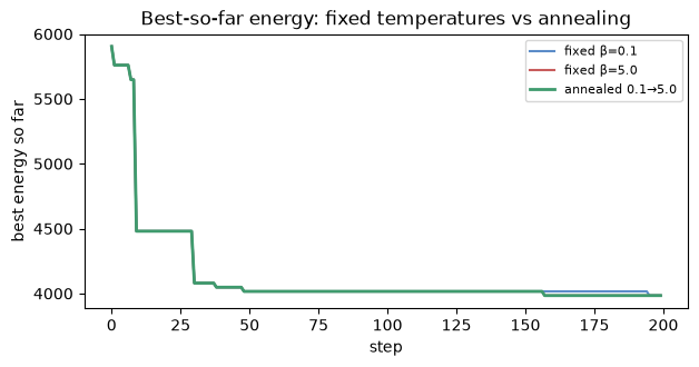
On this small grid all three schedules land close together; on larger instances the annealed schedule typically wins because early exploration escapes the initial partition’s basin before the chain turns greedy. For real experiments use horizons of 10,000+ steps.

Custom acceptance rules

accept is just a callable (proposed: ChainState, current: ChainState) -> bool. You can write your own — for example, threshold-only acceptance for a minimax objective:

def accept_if_below_threshold(proposed, current):
    if not proposed.feasible:
        return False
    max_radius = max(proposed.facility.radii.values())
    return max_radius <= 30.0  # never accept covering radius > 30 minutes

Or a multi-objective rule that requires Pareto improvement:

def accept_pareto(proposed, current):
    if not proposed.feasible:
        return False
    return (
        proposed.energy <= current.energy
        and max(proposed.facility.radii.values())
            <= max(current.facility.radii.values())
    )

SingleMetricOptimizer

For users who want a built-in optimization loop instead of writing the chain manually, SingleMetricOptimizer wraps a chain with simulated annealing and tilted-run schedules.

from falcomchain import SingleMetricOptimizer

def total_radius(partition):
    return sum(partition.facility.radii.values())

opt = SingleMetricOptimizer(
    proposal=partial(hierarchical_recom, epsilon_base=0.3, epsilon_super=0.3, demand_target=1000),
    constraints=lambda p: True,
    initial_state=partition,
    optimization_metric=total_radius,
    maximize=False,
)
# opt.simulated_annealing(...) and opt.tilted_run(...) below

The optimizer tracks opt.best_part and opt.best_score across the run. See the source (optimization.py) for the schedule API — it’s currently undocumented and the surface may evolve.

Energy functions

The default energy is demand-weighted travel time (compute_energy in falcomchain.markovchain.energy):

E(s) = Σ_D Σ_{v ∈ D} d_v · dist(v, f(D))

To use a different objective, pass energy_fn to ChainState.initial. Examples:

• Equity-weighted: weight high-vulnerability units more heavily.

• Max covering radius: minimize the worst district’s radius.

• Compactness penalty: combine travel time with a Polsby-Popper term.

The function signature is energy_fn(state) -> float. It runs once per step (or on demand if cached); for performance-critical objectives you may want to compute deltas instead of the full energy each step (see compute_energy_delta in the same module).

Where to go next

• Running a FalCom Chain — chain mechanics.

• Ensemble Analysis — what to do with the samples.

• Algorithm overview — the four-phase proposal.